Hello! I am a senior in ECE at Cornell interested in firmware and embedded systems. This website will contain updates and overviews of all of the labs for ECE 4160.
Lab 12: Planning and Execution
May 20, 2023
The task of this final lab is to get the robot through a specific path on the map using all of the skills concepts that we have learned this semesters.
Although I felt that localization went well with my robot, I did not have enough time to create a program that would use localization to navigate the map. I decided to use a Feedback Control loop with position control PID to translate the robot on the map, and orientation control PID to rotate the robot.
Feedback Control with PID
To move the robot forward, I used the same PID function from lab 6. I also created a backwards movement function, because there are some points on the map where the wall the robot is facing is too far to make an accurate distance measurement, but the opposite wall from the robot is much closer (like right in the beginning.) This need for backward PID will be discussed more later.
Here are the translational PID functions in my Arduino script. The only difference between the forward and backward functions is which motors are set with nonzero pwm:
To rotate the robot, I tweaked the spin function from lab 11 to have customizable goal angles. I also took out the TOF distance readings, since I am not mapping or localizing.
I also decided to create both a counter-clockwise spin and clockwise spin implementation, so that the robot would never have to turn more than 180 degreed. The larger the turn, the more room for error.
Here is the rotate function:
Here are these PID controls working.
Translational Movement
Code ran in Python:
In lab 6, I set up the PID function to run for 15 seconds, because if I let the function stop when it reached the goal distance, it might not correct itself if it overshot the movement. These movements are not as long as the 2-3 meter long stretch that the robot would move in lab 6, so I probably should have shortened the timer.
Rotational Movement
Code ran in Python:
For some reason, the different directions use different ranges of Kp, the proportional constant. In general, I used larger Kp values for larger rotations. Also, most of the goal degree inputs are not the exact same number as the desired goal. I experimented with all of the rotations, and these were usually accurate, but they worked best on a fully charged battery.
First Try through the Map
At first, I tried to take the shortest path to each next point on the map, and all of the robot translations would be done with the TOF sensor at the front of the body. On my first try, this proved to be a bad idea. When going from point 1 to point 2, the robot would go off full speed towards the wall across the room. I realized that even though the range of the TOF sensor should be 4 meters, the distance to the opposite wall is too far to reliably move forward.
I also thought that getting from position 2 to 3 and 5 to 6 would be too risky. Conveniently, although all of these translations are facing walls that are a bit far away, the walls behind them are much closer. I decided that for all of these legs, I would have the robot move backwards so that the wall distance it was comparing its distance to during PID would be much shorter.
I decided also that starting the map with a rotation of 45 degrees was risky. If the rotation is a little bit off, all of the rest of the translations and rotations will be offset as well. For this reason, I went from position 1 to position 2 by going forward for 2 feet, rotating 90 degrees, then going left for 2 feet. All of the other paths use the shortest path however.
Planned Commands
Here are the functions that I call while the robot moves through the maps.
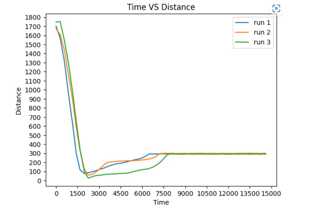
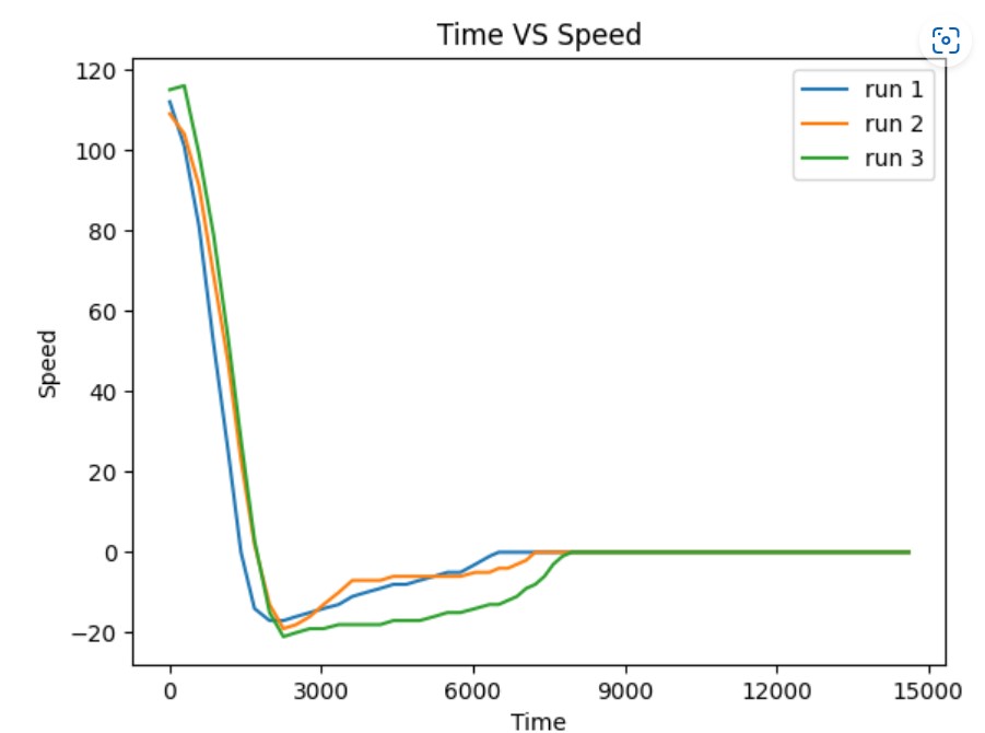
Best Run
Unfortunately, I could not get a video of the robot getting through the entire map, but I got a good run to about the halfway point, and then starting from the halfway point. Here are those videos together. Recall that every translation has a 15 second timer before the next command can be sent.
At the end, I have to intervene and send some custom commands to get the robot to (0,3). I also accidentally sent the wrong direction turn, so I had to continue intervening. Still, it did get to (0,3) eventually, and then had a pretty smooth landing to (0,0).
Even though it took two parts, I am satisfied with how precise the spins and translations are. The day before, the robot was missing most of the goal positions, because either the spin was wrong or the translations would veer to a side.
Final Remarks
What a rewarding lab! This was a hectic finals week for me, and this was the last task I had to do before graduation. Although every lab was challenging and time consuming, I always felt really proud of the robot afterward, which is ultimately my favorite part of engineering.
It would have been cool to implement a closed loop navigation algorithm, but I also think that it's cool that a method without localization could land on all of the waypoints.
One last thank you to Professor Petersen and the TAs who were always willing to help me think through problems or debug. I would not have been able to do most of the labs without the amazing tips and guidance.
Lab 11: Localization (Real!)
May 4, 2023
In this lab, functions to implement localization were provided.
First, I ran the simulation with these functions to make sure that everything was set up correctly. Here is the plot from that:
The program should make the robot spin, get 18 equally spaced distance measurements, and use those measurements to guess where the robot is on the map.
Changing spinning method
First, I changed my Lab 9 code. That program gathered a variable amount of distance measurements, up to 200. I implemented a way for the robot to calculate its current yaw, and only take and store the TOF measurement every 20 degrees of rotation. This method still uses PID to control the angular speed of the robot as it spins. This is a much neater spin, because it spins 360 degrees, then stops.
Here is the code:
Here is a video of the spin:
Note that the robot spins in the counter clockwise direction.
Passing Data through Observation Loop
The Artemis sends back 18 distances and their respective indexes. I used code from Ryan Chan's 2022 website to change the code to fit the given Observation Loop parameters: https://pages.github.coecis.cornell.edu/rc627/ECE-4960/lab12.html
I use a notification handler like in all of the previous labs to receive the data in the Jupyter Notebook, but I could not find a way for the Observation Loop function to both call and receive the data. It wouldn't be able to wait for the notification handler to finish or acknowledge that the global variables existed. Thanks to the advice of the TAs, I decided to call the spin command and store the data outside of the Observation Loop function, and then return the already saved data. Here are these external code blocks and the very simple function:
Running the Localization Commands
With the program implemented, I put the robot in the map and tried it out. Astoundingly, the first two spots that I tried gave me no problems. They correctly guessed the position of the robot. Here are the maps and distance measurement from these runs:
These maps show both the Ground Truth and Belief positions of the robot, but since they are the same positions, only 1 dot is shown. Both of these runs were done with the robot starting facing "up."
For the third position I tried, it first guessed incorrectly:
The Ground Truth is in green, and the Belief is in blue. I wondered if starting with the robot facing the walls would help the program identify that the robot is in a corner, so I tried another run with the robot facing "down" - recall that the robot spins counter clockwise.
This run made the Belief correct!
For the last position, I was not so lucky. I tried several runs with different starting orientations, and the program would guess a position near the Ground Truth, but never the exact Ground Truth. Here is one of those guesses:
I was puzzled by this, because the distance measurements plotted reasonable wall measurements like the other runs. After spending a good amount of time trying to get a good run however, I decided it was time to move on to lab 12.
Final Map
Just for fun, here is the final map of the room from these runs. It is worth noting that this is way better than my map from Lab 9.
Lab 10: Localization Simulator
April 27, 2023
In this lab, we set up and implemented a grid localization simulation using a Bayes Filter. The simulation is done through Jupyter Notebooks. We are simulating localization before implementing it on the real robot to test out the functions in a more stable environment.
The functions I used to do this lab are all from Anya Prabowo's 2022 website: https://anyafp.github.io/ece4960/labs/lab11/
Simulation Set Up
To start the lab, we were given the code to start the simulation and plotting software. These plots looks like this:
Implementions
Now delving into the functions that I used, which again are from Anya's website.
The first function is Compute Control, which computes these equations based on the current and previous position of the robot:
The next function is the Odometry Motion Model, which uses the current and previous postions as well as the control information from Compute Control to output the probability that the robot is in a certain position.
Next, the Prediction Step takes the current and previous odometry readings (the TOF sensor data) to update the current position.
The Sensor Model function returns the probabilities that the sensor measurements the robot collected were correct, given the robot's current pose.
Finally, the Update Step updates the ultimate believed current position.
Video
Now, we can run the simulated robot with this implementation through a preplanned trajectory. In the video, the plotter will show the odometry values(red), the ground truth(green), and the belief(blue) from the filter. With a successful Baye's filter, the belief points should be near the ground truth points.
Lab 9: Mapping
April 20, 2023
Angular PID
To map a room, the robot is place at 5 specified positions throughout the room. In those positions, it will spin 360 degrees, taking distance positions while it spins. Plotting all of these distances should map out the entire room.
For my spinning implementation, I chose angular PID. My angular PID function is based on Anya Prabowo's.(https://anyafp.github.io/ece4960/labs/lab9/)
Here is my implementation:
Here is a video of the robot spinning:
Sanity Check: Polar Plots
I ran the Angular PID at each of the five positions in the room. As a sanity check, I plotted the distances on a polar plot.
I am satisfied with the clarity of the room's corners in these plots. The plots are not oriented in the same way, so I added varying amount of radians to each theta array corresponding to the distances so that the plots would fit together on the final map.
The Map
Next, I had to turn the distance and angle measurements into x and y coordinates. Ryan Chan who took the class last year created a very useful function to complete this task, which I used (https://pages.github.coecis.cornell.edu/rc627/ECE-4960/lab9.html)
In the function, he converts the measurements into x and y coordinates using transformation matrices from Lecture 2 to take the dot product between the distance and the angle.
After some shifting of thetas to align all of the coordinates, here is the final map:
The shape of the room and the box in the upper left corner are pretty defined, but I don't know why the box at the bottom of the room is offset and poorly defined (the edges are rounded.)
Nonetheless, I can draw lines over the coordinates to create a map of the room that will be used by the simulator in lab 10.
Lab 8: Task A Stunt
April 13, 2023
Creating the stunt protocol
Since I chose task A when implementing PID, my robot must do a back flip. In order to do this back flip, the robot drives as quickly as possible toward the wall (without using PID), then before it hits the wall, it suddenly switches to driving backwards as fast as possible.
Here is the Stunt Command protocol in Arduino, using the extrapolation function from lab 7 to estimate when to do the backflip.
Trial Run
Here is the robot doing the backflip and the distance data to go with it.
Here is the robot going back to the starting line but failing to flip. The data for this run was lost.
I was unable to get a run where the robot successfully flips and drives back to the starting line. Also, my TOF sensor was angled upward in a way that was fine for detecting distances from the wall for PID, but when the robot flips over and begins driving backwards, the TOF sensor is angled toward the ground. This angle makes all of the measurements after the flip inaccurate. That is why the distance graph plateaus at a low value at the end of the first run.
Tragedy Strikes
While trying to fix the problem of the TOF pointing at the ground, I was moving around all of the sensors on the robot and something seemed to break.
The program would no longer start because the sensors couldn't be initialized, and I did not have enough time to find the disconnect or resolder the connections.
Lab 7: Kalman Filter
March 30, 2023
Drag and Momentum Estimation
To build the state space for the Kalman Filter, I first found values for drag and momentum, which I will use in my A and B matrices.
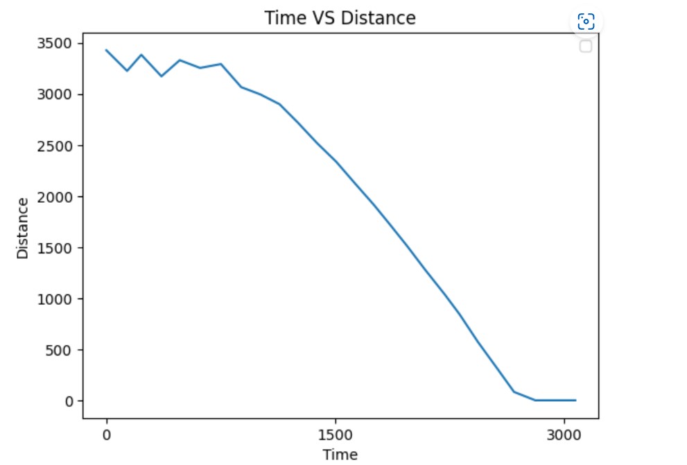
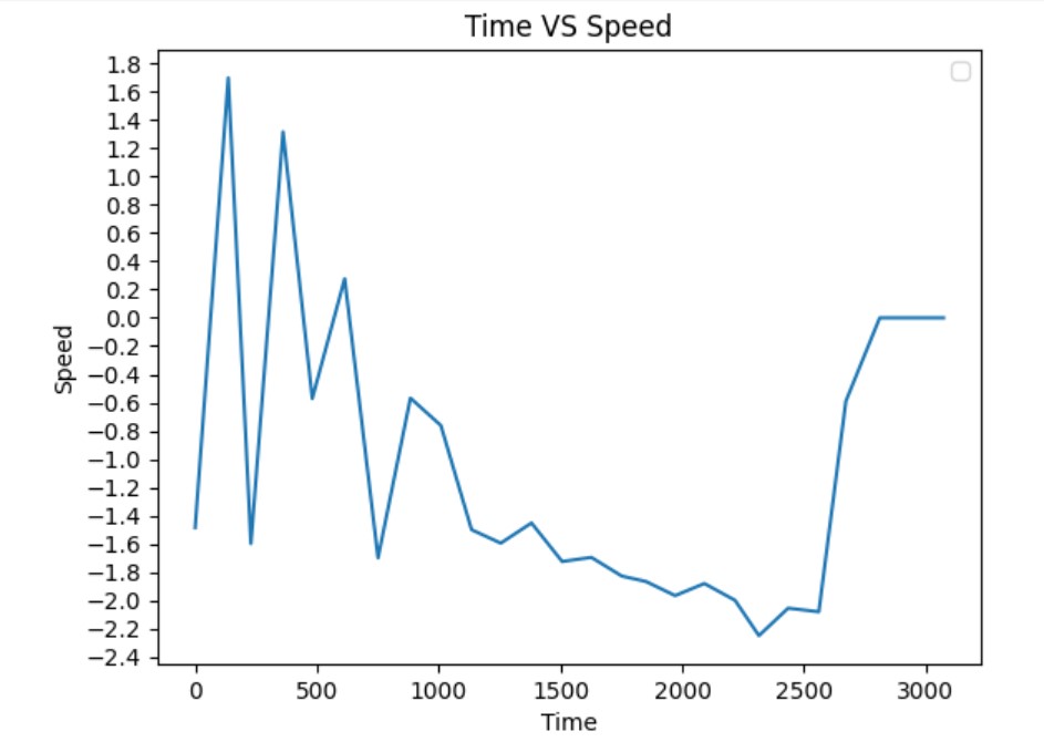
To find these values, I found the steady state speed and the 90% rise time by running the car at a constant PID input of 110, which I found to be the maximum value from lab 6.
Between 2 and 2.5 seconds, the speed oscillates between 2000mm/s, so I take this to be the steady state speed. The speed graph would likely be more smooth if I sampled the distance more often while the car was moving.
90% of the steady state speed is 1800mm/s which occurs at approximately 1.75 seconds.
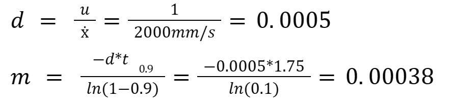
Assuming u is 1, we get these values for drag and momentum:
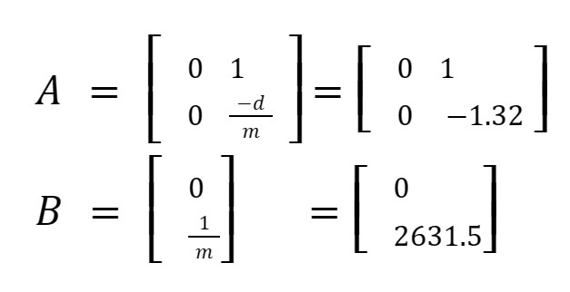
The A and B matrices are therefore:
Sanity Check Kalman Filter through Jupyter
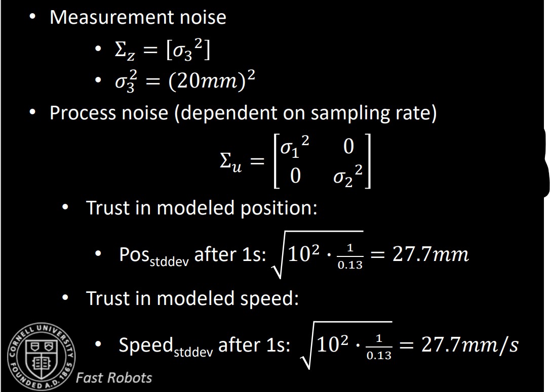
The final values to find before implementing the Kalman Filter are the sigma values, defined in lecture.
My data is sampled about every 0.27 seconds, so I am using 19.24 for my sigma 1 and 2 values. For sigma 3, I use the suggested value of 20.
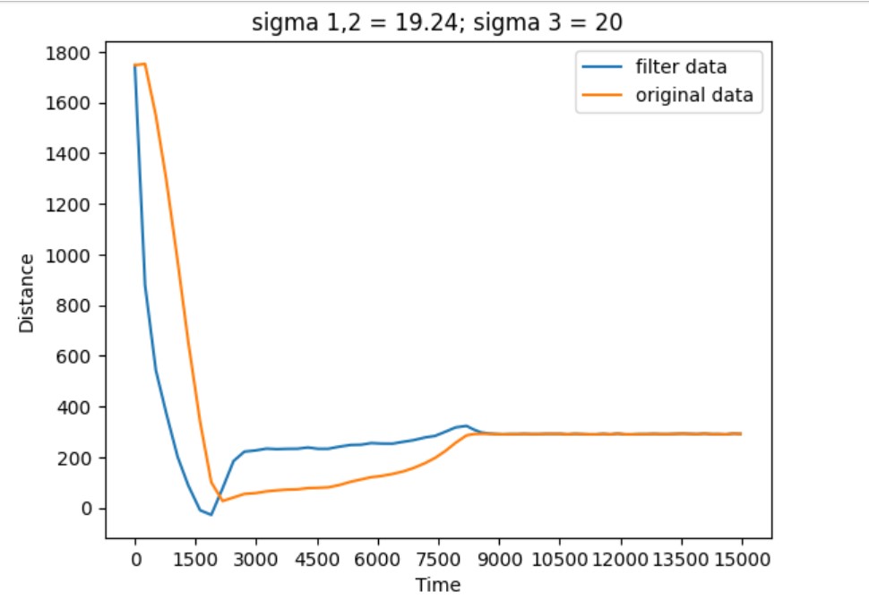
Here is the Kalman Filter setup through Jupyter Lab. I ran the simulation on data saved from a PID run in Lab 6. This program is from Anya Prabowo (https://anyafp.github.io/ece4960/labs/lab7/)
This is what the filter outputs compared to the original data.
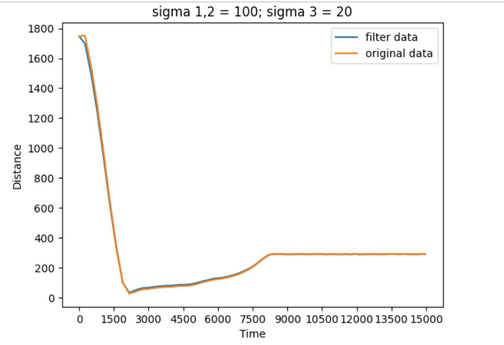
I then tried to amp up the sigma 1 and 2 values up to 100 to see the effects. Increasing these values increases the uncertainty of the model, which means that the values of the sensors would be relied upon more rather than the model.
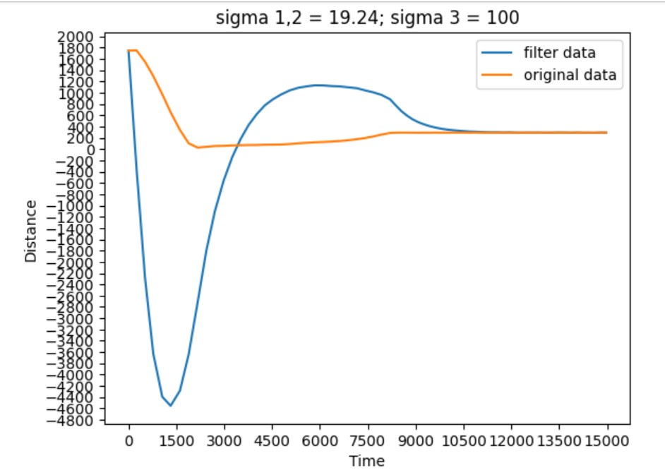
Then I wanted to see what happend with a high sigma 3. Increasing this value does the opposite of the prior test. More trust is put into the model and less onto the sensors.
Ultimately, I will be using the suggested values shown in the first test.
Extrapolation
Since I did not have time to implement the Kalman Filter on the robot, I decided to extrapolate the distance data to estimate when the robot should stop. Here is my extrapolation function and how it is embedded into my PID command:
Here is the extrapolation function working so that the robot stops right before it hits the wall.
Lab 6: PID Control
March 23, 2023
Pre-lab: Sending Data via Bluetooth
For this lab, I wanted to be able to view the distance and speed data of the robot from while it was moving. This means that the Python program will send a PID command to the robot, and then the robot will send back runtime data to the Python program so that I can graph the data.
In previous labs, I sent data to the Python program while it was being collected by the robot. This method is not ideal as using Bluetooth communication while moving and trying to run a control algorithm (PID) can slow down and/or overwhelm the robot, so I shifted to a method where the robot would store the data as it was being collected, and then send it to my computer after it stops moving.
I did not have to change how the Python notification handler works. The biggest change is that I stored the robot data in a 2-dimensional matrix in the Arduino program.
This array stores 150 data points and assumes that one row of time, distance, and speed data is a string of max 30 chars.
During runtime, data is saved one point at a time, then when the robot is done moving, data is sent to the Python program one point at a time. Here is the data being sent:
Now, the notification handler will append to the time, distance, and speed arrays as each data point arrives to my computer. Here is the notification handler in Python:
PID command set up in Arduino
I decided to use PID approach A, which means that the robot will start about 2 meters away from a wall and then move as fast as possible to the wall before stopping right before the wall and backtracking to 300mm away from the wall. I created a PID function which compares the current distance from the wall to the desired distance (300mm). The difference between the two distances is the error, which is multiplied by the proportional constant Kp. The instantaneous derivative of the error is also calculated and then multiplied by the Derivative Constant (Kd.) These two multiplication terms are added together to determine the speed of the motors.
Unless the speed is 0, the value of the speed is never outside of the range [40, 254]. 40 is the minimum PWM I found in lab 5, and 255 is the absolute maximum PWM.
I also use a sampling rate to determine how many data points a 15 second run should store.
The PID command takes in the values of Kp and Kd for easy tweaking. The command protocol collects the distance measurements and then calls PID() for 15 seconds. At the end of these 15 seconds, the robot stops no matter what.
When the robot is done moving, the command finishes by sending over the collected distance and speed data.
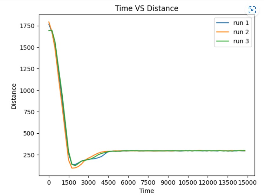
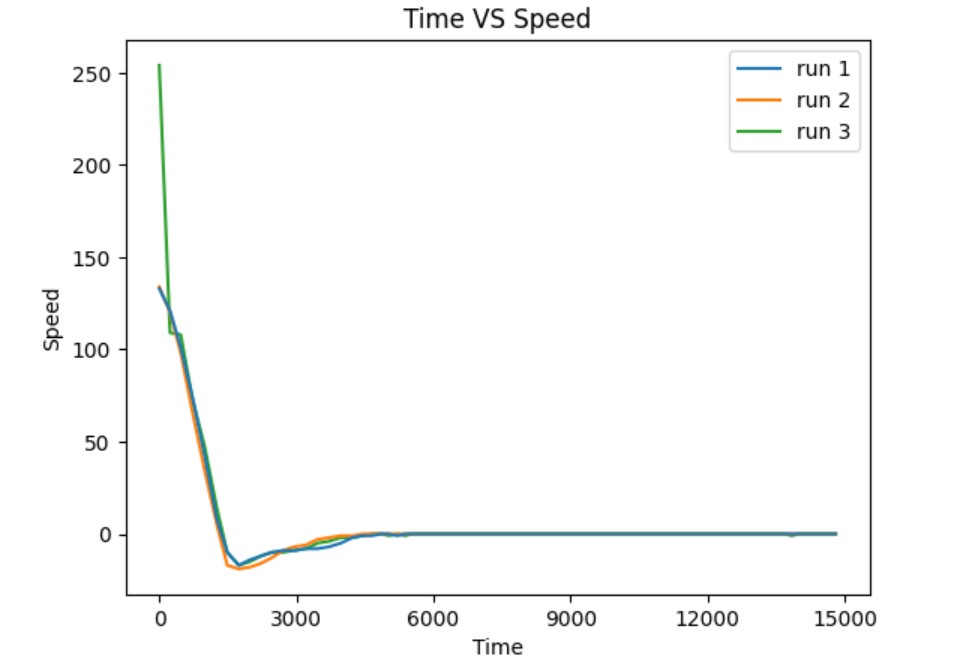
Proportional Constant
First I started off by determining a Kp value without considering Kd. For now Kd = 0. With some experimentation, I came up with a value of Kp = 0.08. This is the highest value I could use before the robot started hitting the wall. Here are the videos and data from 3 runs of the robot using this value with an initial position just short of 2 meters away from the wall. These runs took about 7.5 seconds.
Derivative Constant
With a working proportional constant, it's time to add a derivative constant. This constant will make motor control more powerful by making the error response more adaptive.
I knew that with the derivative constant, I could make the initial speed of the robot faster. I increased the Kp value to 0.09 and started out with a Kd value of 1.5. The run would complete in about 6 seconds, and the robot would not hit the wall. I wanted to see how low I could make Kd before the robot would hit the wall. I ran the command, dropping Kd by 0.01 each time.
I ended up with a Kd value of 0.1 (and Kp of 0.09.) The robot would finish in about 4.5 seconds, a significant decrease from the 7.5 second runs of the solely proportional control runs.
Here are the data and recordings of three runs with these constants.
Lab 5: Starting Motor Control
March 9, 2023
Pre-Lab
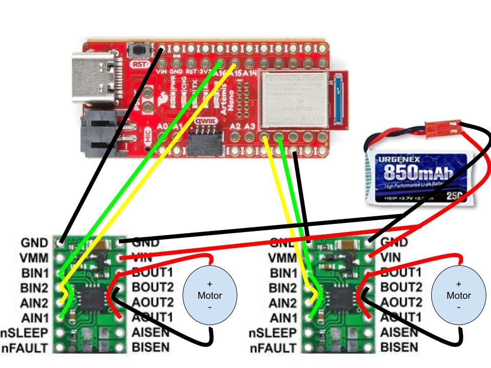
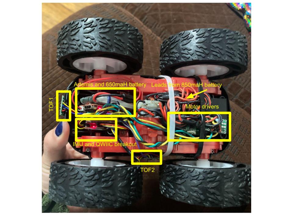
For our system, we are driving each motor with one dual motor driver. To configure this set-up, I wired the chips to be parallel coupled. Here is how the drivers are connected to the Artemis, the motors, and the 850mAH battery:
I based my connections on Ryan Chan's from last year
Recall that the Artemis is powered with a 650mAH battery. The motor drivers will be powered with separate batteries, because motors are so noisy, that it is worthwhile to isolate the motor system as much as possible from the sensors. If the sensors were too physically close to the motor drivers or the motors, or if all of the devices were powered by the same battery, then the sensors and the Artemis could easily pick up unreliable data.
Testing the Motor Drivers
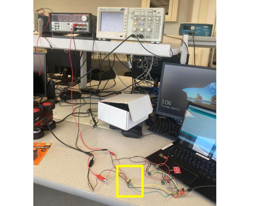
To test this wiring and my soldering skills, before connecting the motors to the drivers, I tested the drivers by inputting PWM signals from the Artemis and viewing the output on an oscilloscope. I powered the driver with a 3.7V signal from the power supply, since this is the voltage supplied by the 850mAH battery that will power them with later.
Here you can see the driver (highlighted in yellow) connected to the Artemis, the oscilloscope, and the power supply.
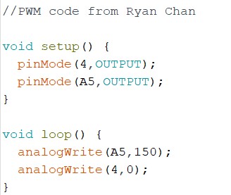
I used PWM code that I found on Ryan Chan's website from last year's class to output a PWM signal from the Artemis.
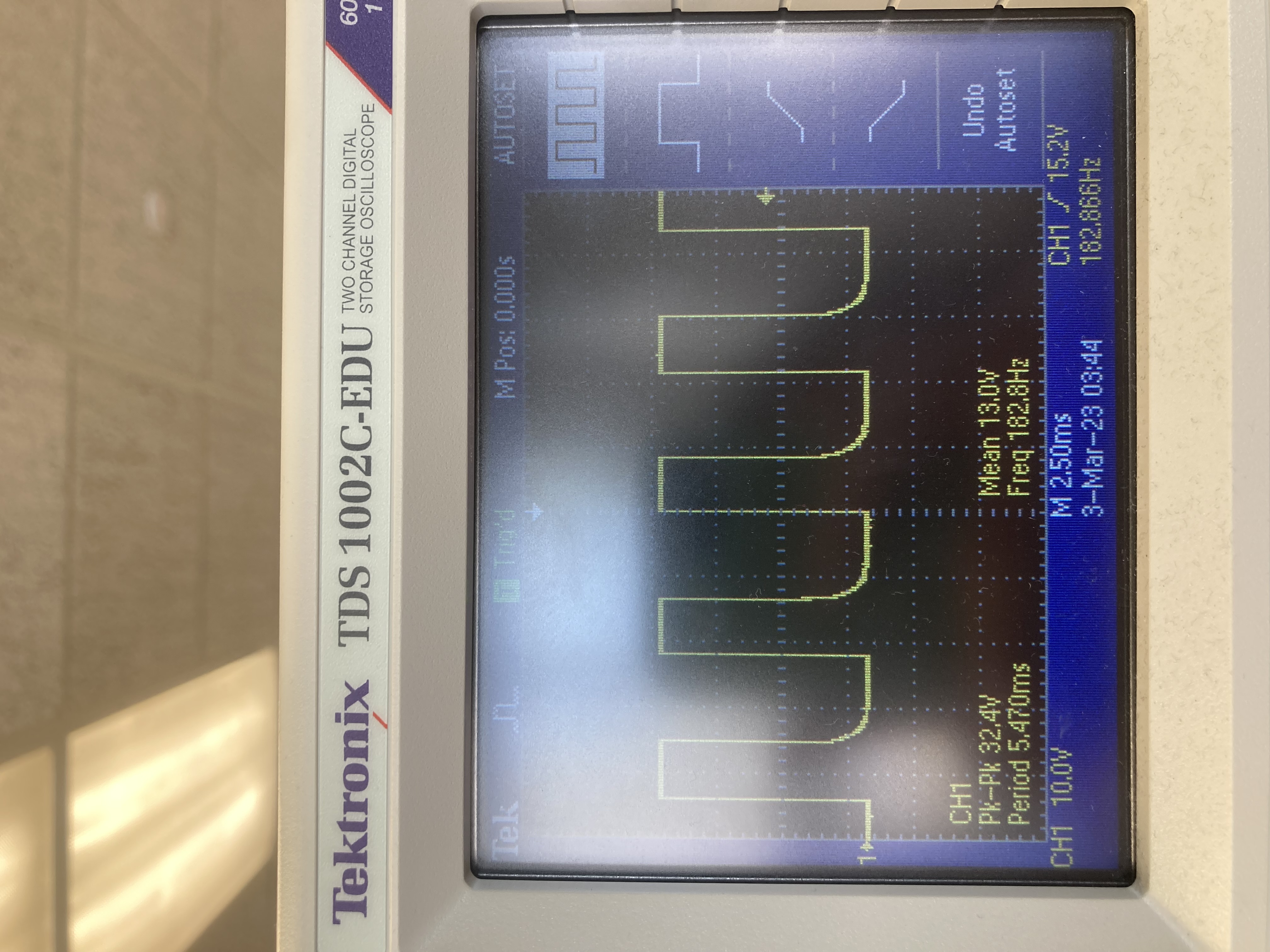
As expected, when driving the driver with PWM inputs, I saw PWM outputs in the oscilloscope.
Testing the Drivers with the Motors
Now instead of viewing the output on the oscillosope, I connected the wires to a motor on the robot. I altered my code so that every 5 seconds the signals from the Artemis were altnerating. This changes the directions of the wheels. Here is the new code:
Here are the wheels turning as expected:
Attaching the components to the Robots
With all of the connections for the drivers soldered, I attached the entire Artemis circuit to the car. My wires are quite long and had to be ziptied to the body, which I might try to change later on.
Running both Motors with the Battery
With the drivers tested, and the car built, here are both sets of wheels spinning. In this set-up, the Artemis and the motor drivers are both powered by their respective batteries. (No more power supply!)
Lower Limit PWM value
The car naturally goes quite fast. With a PWM value range of [0, 255], any number above 100 has the car out of arm's reach within a couple of seconds. With the car working, I tried to find the lowest PWM values that could make the car go forward as slowly as possible.
I did this with a guess-and-check method, increasing the PWM value if the wheels weren't turning continuously and decreasing the PWM values if the wheels were turning too quickly.
I ended up at a value of 50. Here is the robot moving forward with this PWM value.
While it is moving forward, here is what 50 PWM looks like on both sets of wheels:
One set of the wheels is doing most of the work. To combat this and even out the speed of the wheels to acheive smoother forward motions, I callibrated the PWM values by multiplying the PWM of the slower wheels by a factor of the PWM of the faster wheels.
Calibration Factor
I found this calibration factor also by guess and checking, and ended up with PWM values of 70 and 50. This makes the calibration factor 7/5. Here are the wheels running at these values:
Visually, the speeds are more even. Here is the car moving forward for approximately 6 feet:
Here is the code that I used:
Open Loop Control
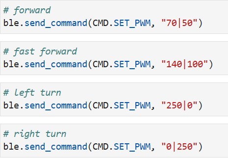
To implement Open Loop control, I added a function to my bluetooth program that I have been writing to in all of the labs called SET_PWM. This function will take two integers as inputs in the Bluetooth Python program, and set them as PWM values for pins 5 and 16 on the Artemis. The robot uses these values for about 2 seconds before stopping. Here is the case statement for this command:
Here is a video demo of the open loop control. I have 4 preset command calls to conveniently move the robot as I desire.
Lab 4: The IMU
February 23, 2023
Introduction
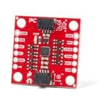
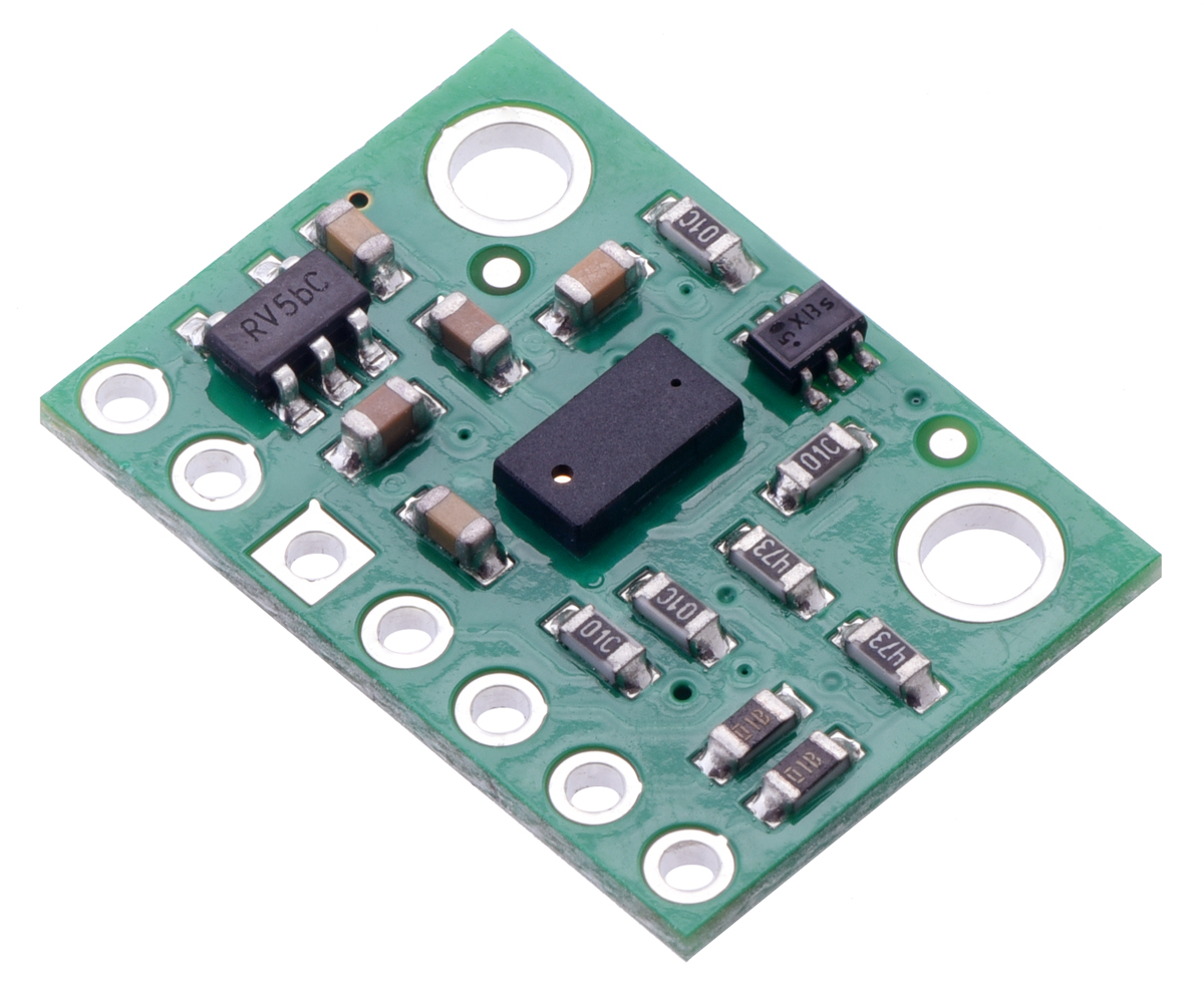
In this lab, we are exploring the uses of an Inertial Measurement Unit (IMU). The sensor we are using is a board from Sparkfun that conveniently connects to the QWIIC breakout board the TOF sensors were connected to in Lab 3.
The Sparkfun IMU board
This IMU contains a "3-axis gyroscope, 3-axis accelerometer, 3-axis compass, and a Digital Motion Processor™" as per the data sheet. For this lab, we will be focusing on the data collected by the accelerometer and the gyroscope.
IMU Set Up
To start, I connected the IMU to the Artemis via a QWIIC connector and the QWIIC connected board.
Since this is a new component, I ran the first Example program in the SparkFun 9DOF IMU Breakout - ICM 20948 - Arduino Library. This program prints out raw data from the gyroscope, accelerometer, and magnetometer. Here is a screenshot of the Serial Monitor while running this example.
In this example program, there is a definition of an AD0 value. This is the value of the last bit of the board's I2C address. By default, this value is 1. When the ADR jumper on the IMU board is closed, then the value becomes 0.
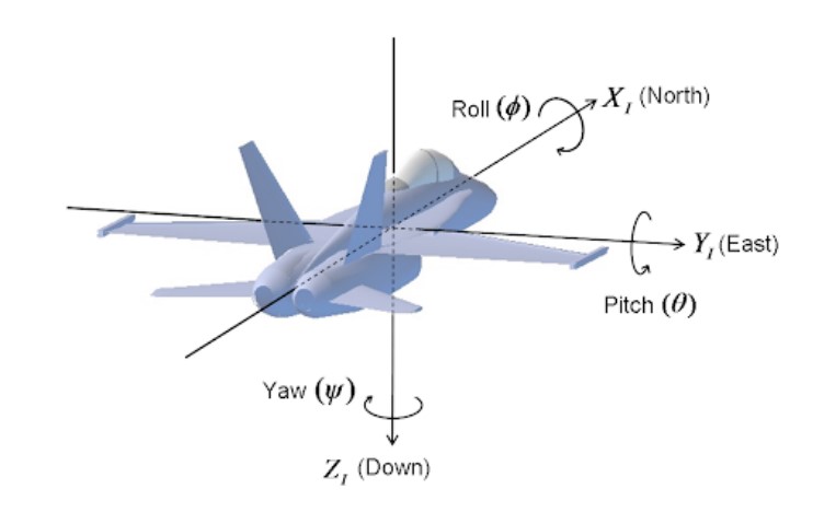
Accelerometers detect linear acceleration, and gyroscopes detect angular velocity. Together the data from these sensors can determine the pitch, roll, and yaw of an object.
diagram from lecture
The Accelerometer
Starting with the Accelerometer, we can start calculating pitch and roll. Using the equations given in the example code from lecture, I calculated these values like this:
I printed these values to the Serial Monitor and tested their accuracy with known angular positions of the board. I used the flat table and the upright side of a sturdy box to represent the 0, 90, and -90 degree angle. Here are screenshots of the Serial monitor during some of this test:
board flat on table
board on its side
board on its other side
While the data is accurate for the most part, it is quite noisy. To quantify this noise, I did a Fast Fourier Transform (FFT) analysis on 1024 pitch data points. I based my program on a Python FFT tutorial.
Here is the FFT graph. While the peak at 0 Hz is clear, there is still a lot of data in the remaining bins.
To combat this noise, I implemented a Low Pass Filter with the code given in lecture. I used 20 Hz as my cut-off frequency.
Here is what the FFT analysis on the pitch looks like with this filter. As you can see, the noise is minimized.
The Gyroscope
While the Low Pass Filter reduced the noise, there could still be less noise. Further more, using a filter like this can be timely and greatly slow down the sampling times of this important data. We can introduce data from the gyroscope and using fusion sensing to get more accurate, less noisy, and smoother data for the pitch and the roll.
First, I again used the example code from class to output pitch, roll, and yaw from the gyroscope alone.
Once again I tested the values of these measurements with known positions of the IMU. As expected, it was noisy.
For sensor fusion, I used the complimentary filter code provided in lecture:
Here is the FFT analysis on the pitch. It shows less noise than the low pass filter.
To further exhibit the benefits of the sensor fusion, here are videos of the filtered pitch and roll outputs alongiside the indivual sensor outputs with known positions of the IMU.
Sample Data
Applying the same approach as Lab 3, I printed the current time using millis() before and after the IMU data was collected.
It takes 3-4 milliseconds to collect the data.
With this information, I made a new command in the program from lab 2 that would collect and send both the TOF and IMU data to my laptop. Here is the case for the command.
The command prints out the data in a similar format as the previous two labs as well. D1 and D2 refer to the two TOF sensors, P is pitch, R is roll, and Y is yaw.
This command sends back 5 seconds of data to my computer. Here is what the collected data looks like:
Connecting the Battery
Now we can start powering the Artemtis with a battery. The car came with 2 650mAH batteries, and our kit came with 1 850mAH battery. Even though the weaker battery came with the car, it makes more sense to use the bigger batter to power the motors. These motors require more power than the board, and later in the semester, the extra time that the bigger battery can offer will be valuable.
To connect the 650mAH battery to the Artemis, I needed to cut the plug-in connected off of the battery and solder the wires to a connector that fits into the board. I cut and soldered carefully, working on one wire at a time and using Heat Shrink. Here is the finished battery connected to the Artemis.
Stunt!
It's time to play with the car! First, I powered on the car and its remote and played around with the controls to see what the body was capable of.
It was a lot of fun to play with the car. It moved a lot faster than I thought it would, and it is pretty powerful. I enjoyed making it do flips by switching directions quickly. Also, it is very good at spinning in place.
With some experience with the car, I secured the Artemis and the sensors onto the car (temporarily for now) with zip ties and tape, and I ran the TOF and IMU data collection command while driving forward then spinning.
Here are the distance and IMU data graphs over time from this run.
Lab 3: Time of Flight Sensors
February 16, 2023
Pre-Lab
Time of Flight sensors are used to detect how far something is, such as a wall. The final robot will use two of these sensors.
picture from Polulu
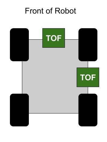
With two sensors, it is worthwhile to consider where on the robot's body the sensors will be placed. It is natural to put one sensor at the front of the robot so that it does not hit walls head on. After that, I will put the other sensor on the right side of the robot.
This side sensor will help detect when to take a turn. If it is at a corner where both the right and front sensors are detecting a close wall, it should take a left turn. If it was just in a region where the right wall was close and now it is far, maybe it should take a right turn. There would be better mobility with a third TOF sensor on the left side, but when the sensors are actually on the robot I can play around more with their placements.
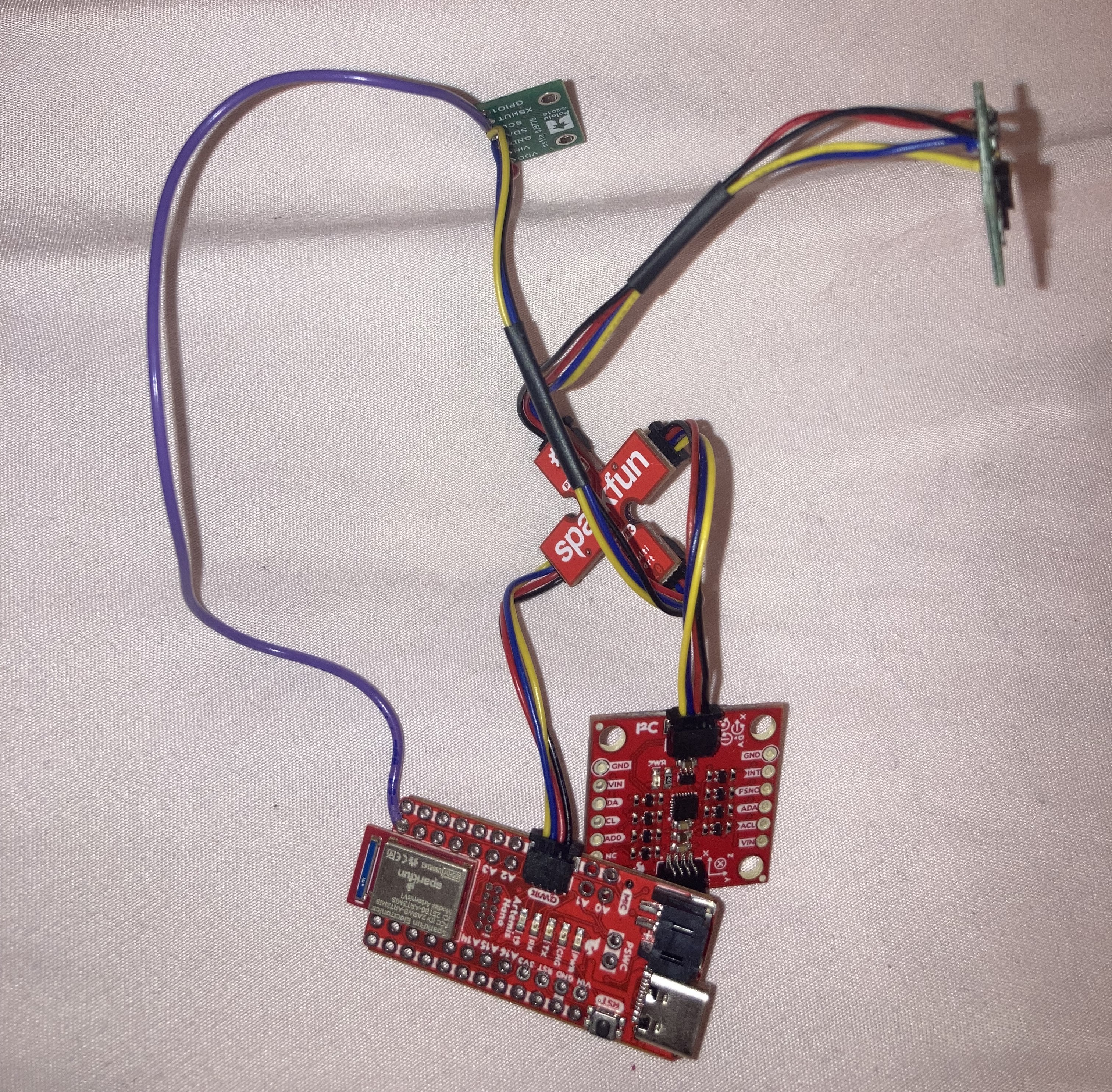
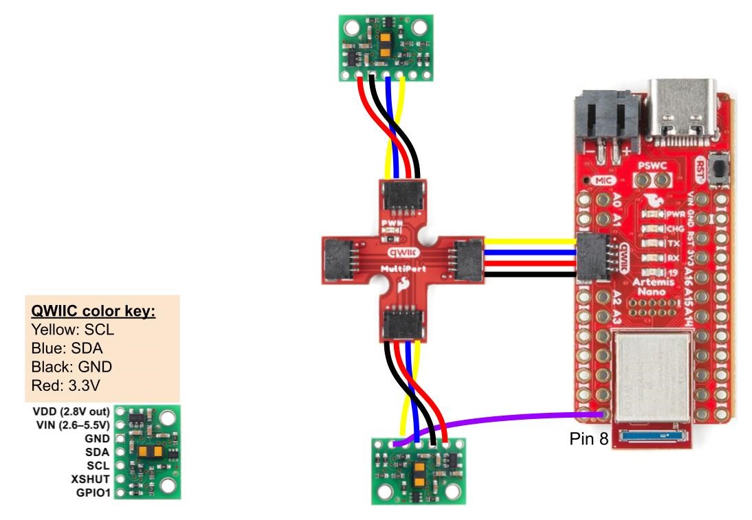
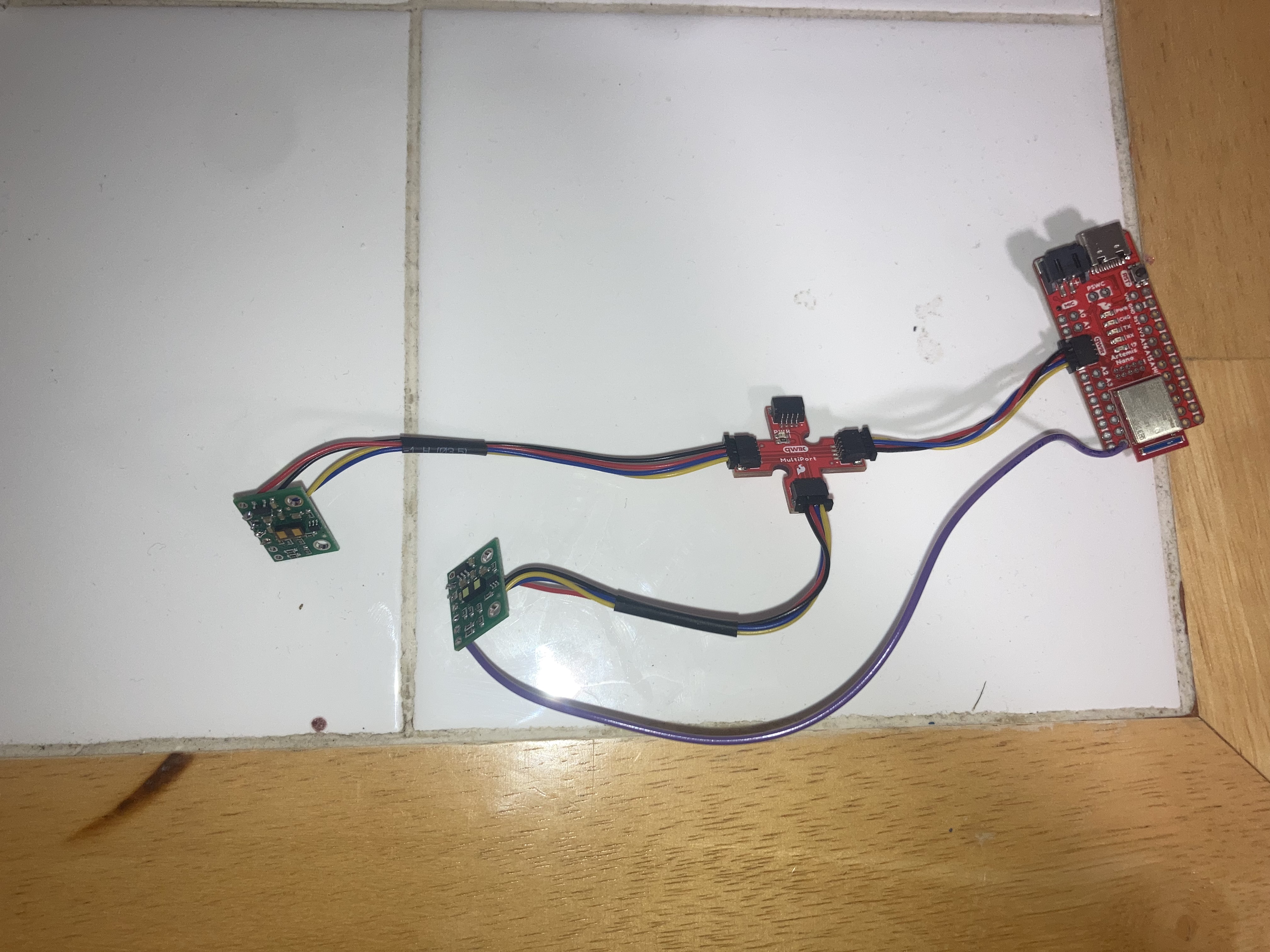
The sensors communicate with the Artemis via I2C. To wire this system, I used a QWIIC breakout board from Sparkfun, and soldered the ends of the QWIIC cables to the TOF sensors. I also connected the XSHUT pin of one of the TOF sensors to a GPIO pin on the Artemis so that data can be read from both, which will be discussed more later in this write-up.
Here is what the actual circuit looks like:
Using One Sensor: Sensor Address
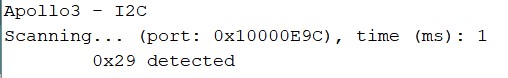
Before jumping straight to getting data from both TOF sensors simultaneously, I started out by checking the address of the device with the Wire_I2C example program in the Apollo3 library.
The address is 0x29. This address is how the Artemis will identify which device it is exchanging data with on the I2C SDA line.
Reading data from the Sensor
Now to read distance data from the sensor, I ran the Read Distance example program from the SparkFun VL53L1X 4m Laser Distance Sensor Library.
There are two modes to choose from: Short (max range is 1.3m) or Long (max range is 4m). For the purposes of this class, I chose the short distance mode. 4 meters is a long distance, especially to our relatively small robots (the sides are less than a foot long). Also, for the sake of not running into things, I want the robots to be able to accurately detect obstacles that are closer than 2 feet away.
The Long Distance mode is the default mode, so in the setup of the Arduino program, I called the function .setDistanceModeShort().
To test the sensor's accuracy, I collected several of it's readings at known distances.
The sensor was very accurate up to about 2 feet away. Then it began underestimating increasingly. At 3.5 feet away, it read 3.14 feet away. This is manageable, and when using the sensors on the robot in the future, I will be cautious and take these underestimations into account.
Two Sensors in Parallel
The two TOF sensors have the same address. For the Artemis to be able to communicate with both chips in parallel, either the sensors need to alternate turning on and off during each read, or one of them needs a different address.
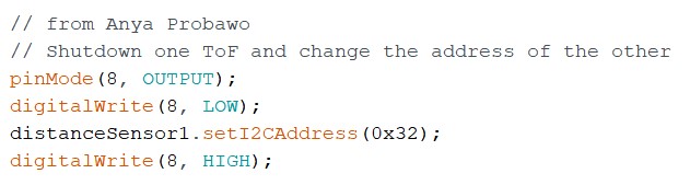
Basing my approach on Anya Probawo's Write Up from last year, I decided to change the address of one of the sensors. I soldered a wire from the XSHUT pin of one of the sensors to GPIO pin 8 on the Artemis. This wire allows me to shut down one of the sensors. During this shutdown in the setup of the Arduino program, I set the address of one of the sensors to 0x32.
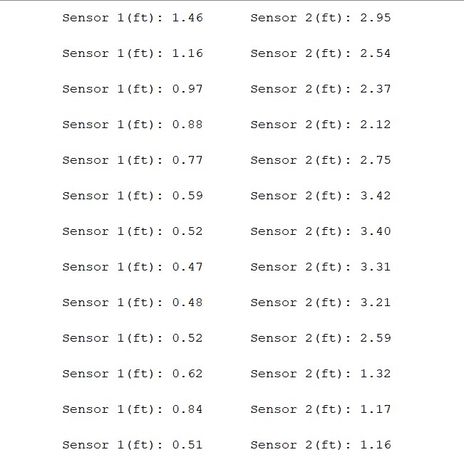
Now the Artemis can communicate with both sensors without any mixup. Here are the readings from the sensors.
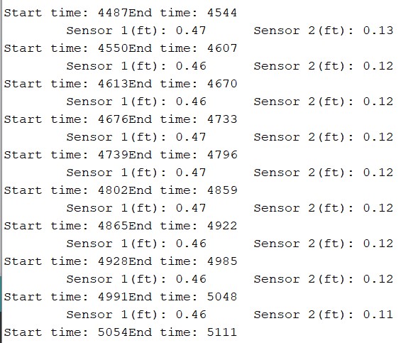
Timing of Data Reading
Now we are interested in how long these sensor readings take. I read the time using millis() before the data was taken and again right after it was taken.
It can be seen that each reading takes 57 milliseconds. The bulk of this delay is from the sensor itself collecting data. If less data was collected, the delay would be shorter, but the results would be less accurate.
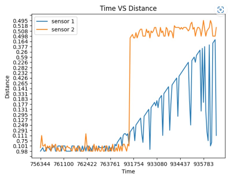
Time Vs. Distance
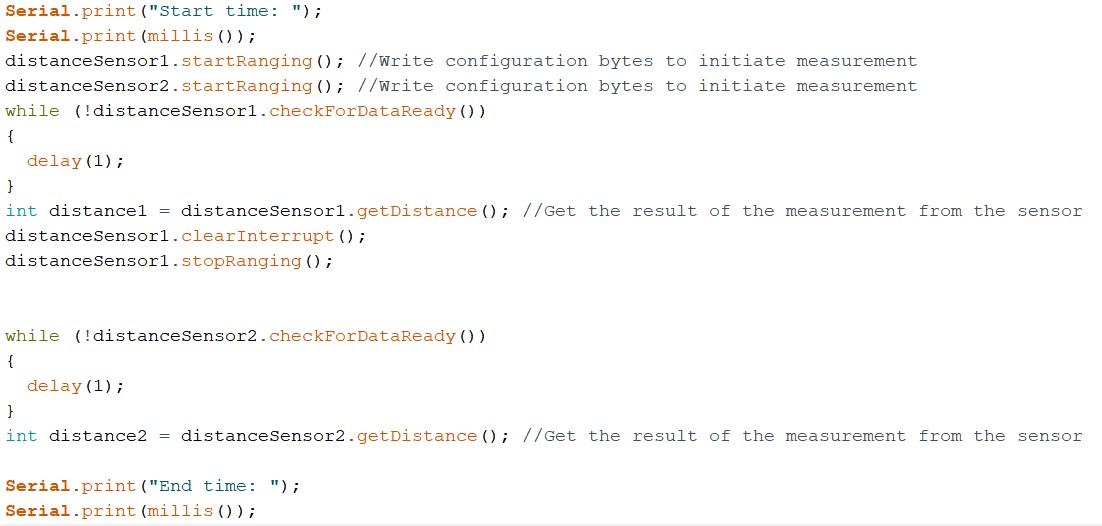
With the sensors working, we can send their data to my laptop via Bluetooth using the command protocol from lab 2. I started out by creating a GET_TOF command.
The current time and two distance data points are sent to my laptop in the form of "T:(time)|D1:(distance1)|D2:(distance2)
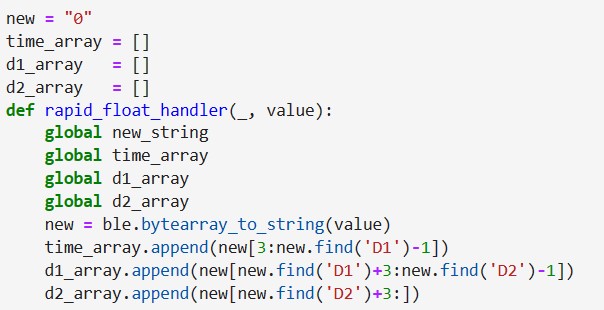
Then I modified the notification handler to read the individual data points and append them to their respective arrays.
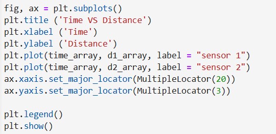
With the arrays set up, I plotted them using MatPlotLib
Lab 2: Bluetooth Configuration with personal laptop
February 8, 2023
Pre-Lab
The set up for this Bluetooth lab requires running a python script on a computer and an Arduino sketch on the Artemis. To run the Python scripts, we are using a virtual environment software called Jupyter Lab. When Bluetooth is configured, the Python program running on my computer can send any of a set of fixed commands to and receive a response from the Artemis.
There was some struggle with getting this system set up, but thanks to the wonderful TAs and collaborative efforts on Ed Discussion, a solution to setting up Jupyter Lab on Windows 11 was found using Windows Subsystem for Linux (WSL).
We were given a Codebase for this lab which provided both a Python and an Arduino demo, and could already send a few commands and messages between the devices.
Before sending any commands or messages to each other, the devices must establish a connection. This is done with the Artemis's MAC address and a few common Universally Unique Identifiers (UUIDs.)
Configurations
The first step was finding the Artemis's MAC address. Upon running the given Arduino program, the device's MAC address is printed in the Serial Monitor. This MAC address is then stored in connections.yaml on the Python side so that my laptop will know which device to search for.
I then generated a new UUID and stored it in both the Python and Arduino Programs
Going through demo.ipynb
With the Configuration set up, I went through the provided Python demo program to verify that the connection was working before trying to change or write any new code. Here is a video of a successful run through the demo.
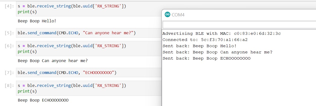
ECHO command
After successfully getting through the demo, it was time to implement my own commands starting with an ECHO command. The Python program sends this command along with a string, and the Arduino should Echo the string back. Here is my code for how the Arduino handles an ECHO command:
To verify, here is what the response looks like in the the Serial Monitor and Jupyter Lab.
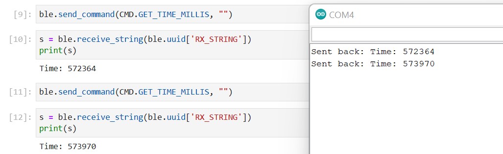
Get Time Comand
To implement a command that returns a time stamp, I use an Arduino function called millis() which returns the number of milliseconds that have passed since the Arduino last restarted.
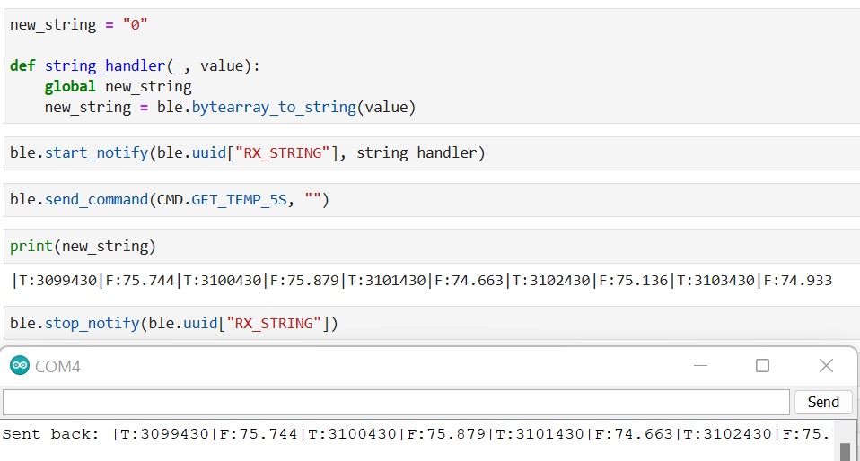
Notification Handler
Now that implementing commands is more natural, it is helpful to set up a notification handler, such that the string received form the Arduino can be received automatically (Notice that in the previous two examples I had to store the string into a variable "s" manually.)
For notifications I make use of two already existing functions: start_notify() and stop_notify(). Calling start_notify() requires a notification handler. This is a callback function which automatically stores the received string. To see what the notification handler has stored, I print that variable. Here is the notification handler working with the GET_TIME_MILLIS command that we got working earlier.
To stop the notification handler, you just call stop_notify().
Get Temperature Comand
Now let's start sending data from the Artemis to my laptop. Using the temperature reading setup from the Analog_Read example sketch (See Lab 1), here is the code for a Get Temperature command:
This program samples the temperature sensor every second for 5 seconds, and then sends all 5 samples as well as their timestamps back to my laptop.
RAPID Get Temperature Command
What if samples came into to my laptop much quicker than once a second? Most likely, they will. This final command will request as many samples as the Artemis can send in 5 seconds. Here is the Arduino code for it:
Instead of concatenating all of the samples within the Arduino progam like I did in the previous command protocol, the board sends each sample one at a time. This is because we have defined the maximum character count for a sent string to be 151. With variable lengths of time stamps, it is safer to send one sample at a time, especially when you have a notification handler that will be able to store all of the incoming values.
I created a new RAPID notification handler, which appends all of the incoming strings into one long string. Here is the new notification handler in action:
As you can see, you can check on the strings while the command is still sending over the data. Also, the final data samples are the same, verifying that the notification handler worked properly.
Limitations
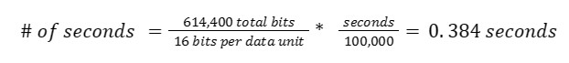
Before getting too excited about sending hoards of information back and forth between my laptop and the Artemis, it is important to consider what the Artemis can handle. The board has 384 kBytes of RAM, which is 3,072,000 bits. This is how many bits the board could send at one time before something bad happens (maybe the board crashes, the Bluetooth connection is lost, etc.) Let's consider what this amount of RAM could send.
To be safe, let's use 20% of the RAM for Bluetooth communication. The board could be using its RAM for many other things. 20% is 614,400 bits.
Looking ahead to Lab 3, the fastest I2C frequency of the Time of Flight sensors that we will be using is 400kHz. Let's consider a frequency of 100kHz. Asumming that data is sent in units of 2 bytes (16 bits), we could store data on the Artemis for 0.384 seconds befores sending it to my laptop.
With smaller frequencies, we could store data for longer periods of time (proportionally). Recall that when the frequency was 1 Hz for the original GET TEMP command, we stored data for 5 seconds with no problem. If we knew we could use more RAM we could store data for longer as well, but again, if we have a notification handler, we could make the laptop do the work of appending the samples.
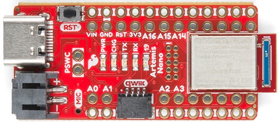
Lab 1: Introduction to the Redboard Artemis Nano
February 1, 2023
This first lab helped with becoming familiar with the Artemis board and
uploading Arduino programs to it. After setting up the Arduino IDE on a lab computer,
I ran 4 pre-written example programs on the board.
Redboard Artemis Nano picture from Sparkfun website
Example Program 1: Blinking Light
The simplest program to run on any board is blinking an LED.
Similar to outputting "Hello World," this program ensures that the system is set up properly.
Example Program 2: Serial Monitor
This next example tests the serial communication feature of the board.
Upon running this program, a series of print statements appear in the Serial Monitor.
Example Program 3: Analog Read
Now testing the onboard testing sensor. Notice how in the beginning of the video,
the temperature values are in the 32,200 count range. After I press my thumb onto the board, heating it up,
the temperature increases to the 32,600 count range. After I release my thumb, the temperature drops back down to 32,200 counts.
Example Program 4: PDM
The final example tests the microphone capabilities of the board. The Serial Monitor prints out the
frequency the microphone detects, and when I whistle into the microphone, the frequency skyrockets to the 2000 Hz range.